How to fit xsdm models with species occurrence data using xsdm

\[ \newcommand{\mean}[1]{\overline{#1}} \newcommand{\var}{\text{var}} \newcommand{\cov}{\text{cov}} \newcommand{\cor}{\text{cor}} \newcommand{\Rp}{\text{Re}} \newcommand{\E}{\text{E}} \newcommand{\ltsgr}{\text{ltsgr}} \newcommand{\expit}{\text{expit}} \newcommand{\logit}{\text{logit}} \]

Abstract. This document introduces the statistically and computationally sophisticated user to the main functions of the xsdm package. Some users may choose to read the document entitled “The xsdm statistical model” prior to reading this document, but it should also be possible to start here. The xsdm package implements a frequentist analysis of the xsdm model. This document should get the user to the point of maximizing the likelihood of the model and profiling in “easy” cases, with callouts to other documents which can help you decide what to do when the process does not go so smoothly. Alternative fitted models can also be compared by AIC or another criterion. The example worked out here is for a virtual species (i.e., generated data), so we also demonstrate that fitting an xsdm model can recover the true parameters if model mis-specification is not an issue.

Introduction to the running example used throughout this document

This manual uses a small built-in example included with the xsdm R package to illustrate a baseline workflow. The example contains (i) an occurrence table for a virtual species, and (ii) two environmental terra raster time series representing CHELSA-derived bioclimatic variables for a region of interest over 39 years.

Load the data and get oriented to the first bioclimatic variable, which is mean annual temperature in units of \(100 \times ^\circ\)C for 39 years for a particular region of interest. And make it units of \(^\circ\)C:

library(xsdm)

bio_1 <- terra::unwrap(example_1$bio01)
class(bio_1)

## [1] "SpatRaster"
## attr(,"package")
## [1] "terra"

dim(bio_1)

## [1] 128 123  39

mm <- terra::global(bio_1,fun=c("min","max"))
min(mm$min) #global min over all years and all locations

## [1] -154

max(mm$max) #global max

## [1] 2061

bio_1 <- bio_1/100 #Make it degrees C

Now load the second environmental variable, which is annual total precipitation, in units of kg/m\(^2\), for the same 39 years and the same region of interest:

bio_12 <- terra::unwrap(example_1$bio12)
class(bio_12)

## [1] "SpatRaster"
## attr(,"package")
## [1] "terra"

dim(bio_12)

## [1] 128 123  39

mm <- terra::global(bio_12,fun=c("min","max"))
min(mm$min) #again the global min, all years and locations

## [1] 45

max(mm$max) #global max

## [1] 1761

If the scales of your environmental variables are vastly different, it can cause problems with optimization. So we change the units for precipitation to make the range of values similar to those for temperature. Now the units are going to be dg/m\(^2\):

bio_12 <- bio_12/100
mm <- terra::global(bio_1,fun=c("min","max"))
min(mm$min)

## [1] -1.54

max(mm$max)

## [1] 20.61

mm <- terra::global(bio_12,fun=c("min","max"))
min(mm$min)

## [1] 0.45

max(mm$max)

## [1] 17.61

Next load data on detections and non-detections/pseudo-absences for a species:

d <- example_1$occ_df
class(d)

## [1] "tbl_df"     "tbl"        "data.frame"

dim(d)

## [1] 4000    4

head(d)

##                name      lon     lat presence
## 1 Species virtualis -1108723 1402222        1
## 2 Species virtualis  -883723 1402222        0
## 3 Species virtualis  -808723 1422222        1
## 4 Species virtualis -1168723 1552222        0
## 5 Species virtualis -1028723 1437222        0
## 6 Species virtualis  -948723 1452222        1

sum(d$presence==1)

## [1] 1609

Now take a basic look at the environmental variables and the species data, just to see what we have. Start by getting the means through time of the environmental time series and plotting:

m_bio_1 <- terra::app(bio_1,mean)
m_bio_12 <- terra::app(bio_12,mean)
par(mfrow=c(1,2))
terra::plot(m_bio_1,axes=TRUE,main="Mean, bio1",xlab="x",ylab="y",legend=TRUE)
terra::plot(m_bio_12,axes=TRUE,main="Mean, bio12",xlab="x",ylab="y",legend=TRUE)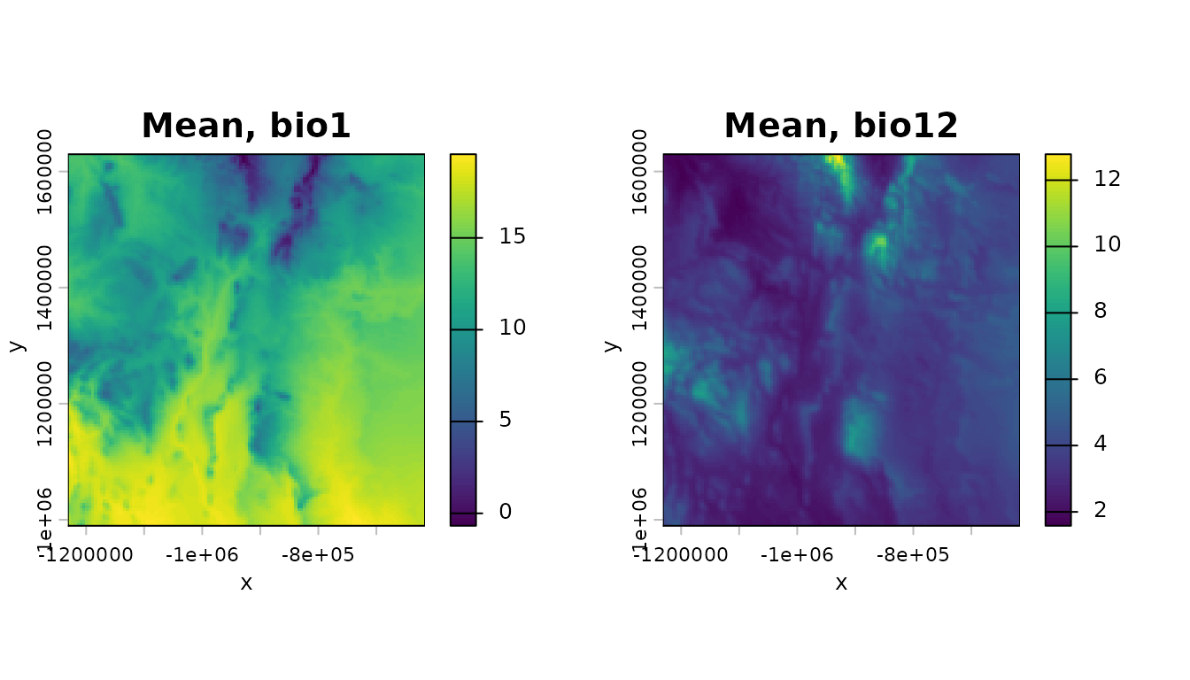

Now do the same for standard deviations:

sd_bio_1 <- terra::app(bio_1,sd)
sd_bio_12 <- terra::app(bio_12,sd)
par(mfrow=c(1,2))
terra::plot(sd_bio_1,axes=TRUE,main="SD, bio1",xlab="x",ylab="y",legend=TRUE)
terra::plot(sd_bio_12,axes=TRUE,main="SD, bio12",xlab="x",ylab="y",legend=TRUE)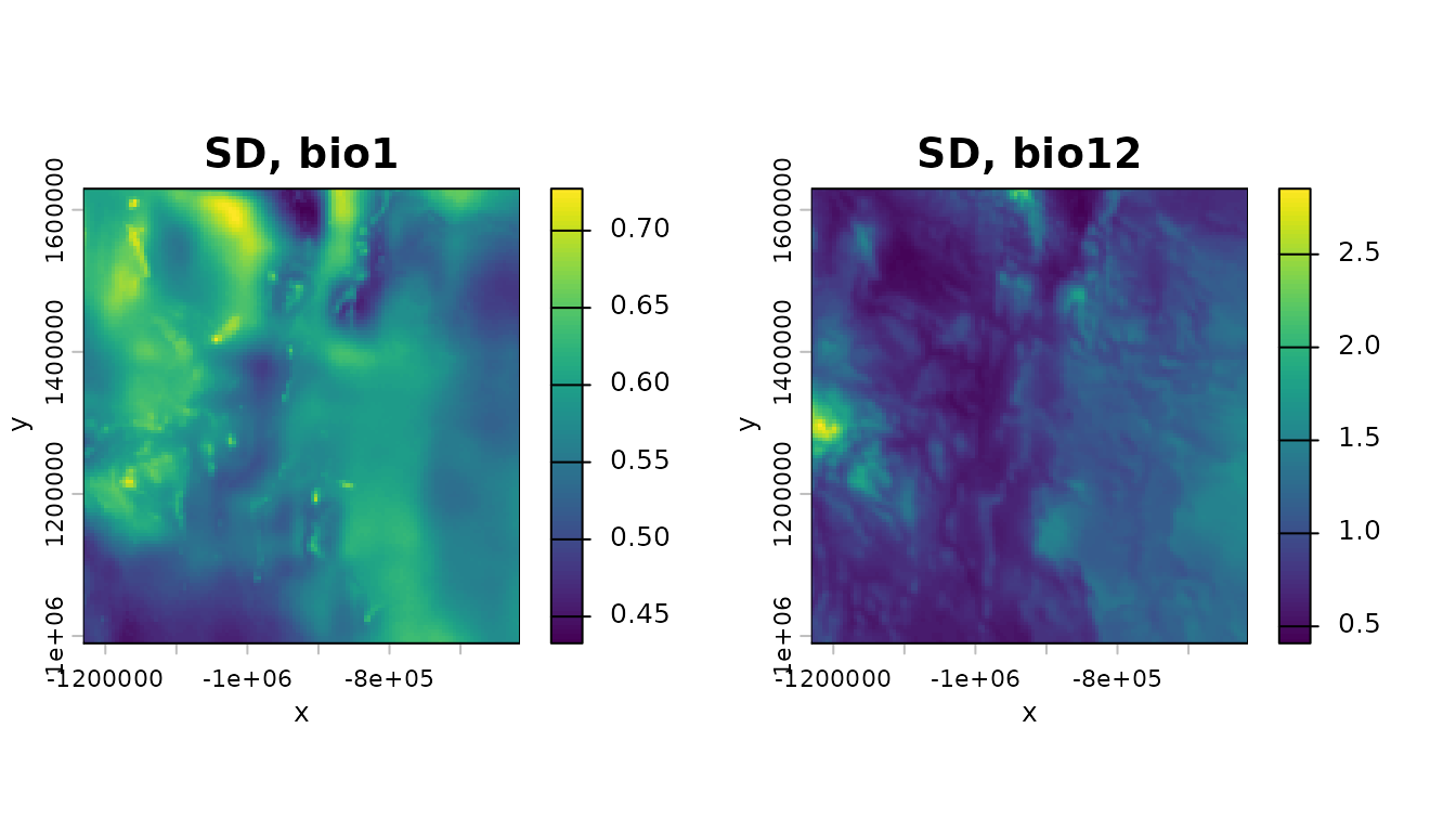

Now plot the species detections and non-detections/pseudo-absences on a backdrop of the mean of bio 1:

pts_0 <- terra::vect(as.data.frame(d[d$presence==0,]),geom=c("lon","lat"),crs=terra::crs(m_bio_1))
pts_1 <- terra::vect(as.data.frame(d[d$presence==1,]),geom=c("lon","lat"),crs=terra::crs(m_bio_1))
par(mfrow=c(1,2))
terra::plot(m_bio_1,axes=TRUE,main="Non-detections",xlab="x",ylab="y",legend=TRUE)
terra::plot(pts_0,add=TRUE,col="black",pch=20,cex=.2)
terra::plot(m_bio_1,axes=TRUE,main="Detections",xlab="x",ylab="y",legend=TRUE)
terra::plot(pts_1,add=TRUE,col="black",pch=20,cex=.2)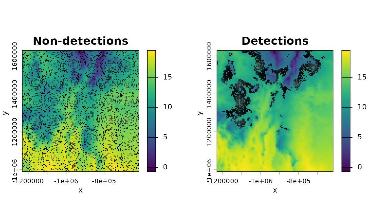

The fitting tools offered by xsdm use a more succinct version of the data, since only the environmental time series at the locations for which there is a detection or a non-detection/pseudo-absence matter; though we will return to using rasters after fitting and model selection. So, for now, we cut out only those time series at the species locations and store them in an array using the convenience function env_data_array():

env_data <- list(bio_1=bio_1, bio_12=bio_12)  # order defines variable 1 and 2
env_array <- env_data_array(env_data, d)  # (n locations) x (time) x (p vars)
class(env_array)

## [1] "array"

dim(env_array)

## [1] 4000   39    2

And we pull out the presences/pseudo-absences as a binary vector:

occ <- d$presence
length(occ)

## [1] 4000

Now we are ready to think about how the xsdm model applies to our data.

Evaluating the likelihood

The xsdm model’s likelihood function is described in the document “The xsdm statistical model”, where model parameters are also described in detail. Parameters are:

\(\vec{\mu}\), which encodes ideal values for population growth of the two environmental variables (a length-2 vector for the present scenario of two environmental variables, unconstrained values);
\(\tilde{\vec{\sigma}}_L\), which has to do with breadth of the growth-environment function “to the left” with respect to two basis vectors (a length-2 vector for our case, positive entries);
\(\tilde{\vec{\sigma}}_R\), which is similar but “to the right” (a length-2 vector, positive entries);
\(\tilde{c}\) and \(p_d\), which relate to species detection (scalars, \(\tilde{c}\) is unconstrained and \(0<p_d\leq 1\)); and
\(O\), which is an orthogonal matrix which describes the basis vectors mentioned above (\(2 \times 2\) for the present example, must be orthogonal, i.e., \(OO^{\tau}=I\) for \(\tau\) the transpose).

In code, the above parameters are denoted mu, sigltil, sigrtil, ctil, pd, and o_mat.

The likelihood is coded as loglik_bio(), so as an introduction to the function let’s evaluate it at a haphazardly chosen set of parameters:

mu <- c(1,1)
sigltil <- c(1,4)
sigrtil <- c(2,3)
ctil <- -10
pd <- 0.8
o_mat <- diag(2)
loglik_bio(env_array,occ,mu,sigltil,sigrtil,o_mat,ctil,pd)

## [1] -2110.297

By default, the function gives the log likelihood, but you can also get the linear-scale likelihood:

loglik_bio(env_array,occ,mu,sigltil,sigrtil,o_mat,ctil,pd,return_prob=TRUE)

## [1] 0

For these haphazardly chosen parameters, the (linear-scale) likelihood is zero to within numeric precision - this is typical. We next optimize.

An unconstrained parameter space

Some model parameters are constrained, i.e., only certain values are allowed (specifically, sigltil, sigrtil, pd, and o_mat; see previous section). Rather than attempt to perform optimizations subject to these constraints, we here define a transformation from an unconstrained Euclidean space to the space of allowed parameters, and we subsequently optimize on the unconstrained space. Parameters in the unconstrained space are henceforth called “math-scale” parameters, and the constrained parameters described above are called “biological-scale” parameters because they more directly represent biological quantities. When a distinction is needed in mathematical notation, we denote biological-scale parameters with a superscript \((b)\), and math-scale parameters with a superscript \((m)\), i.e., \(\vec{\mu}^{(b)}\), \(O^{(b)}\), \(\tilde{\vec{\sigma}}_L^{(b)}\), \(\tilde{\vec{\sigma}}_R^{(b)}\), \(\tilde{c}^{(b)}\), and \(p_d^{(b)}\) versus \(\vec{\mu}^{(m)}\), \(O^{(m)}\), \(\tilde{\vec{\sigma}}_L^{(m)}\), \(\tilde{\vec{\sigma}}_R^{(m)}\), \(\tilde{c}^{(m)}\), and \(p_d^{(m)}\).

The transformation from math- to biological-scale parameters acts separately on each parameter, as follows for all the parameters except \(O\):

\[ \begin{aligned} \vec{\mu}^{(b)} &= \vec{\mu}^{(m)} \\ \tilde{\vec{\sigma}}_L^{(b)} &= \exp(\tilde{\vec{\sigma}}_L^{(m)}) \\ \tilde{\vec{\sigma}}_R^{(b)} &= \exp(\tilde{\vec{\sigma}}_R^{(m)}) \\ \tilde{c}^{(b)} &= \tilde{c}^{(m)} \\ p_d^{(b)} &= \expit(p_d^{(m)}). \end{aligned} \]

Here, \(\exp\) of a vector is interpreted to be the vector resulting from \(\exp\)-transforming each component, and \(\expit\) is the standard logistic sigmoid function \(1/(1+\exp(-x))\), i.e., the inverse of the \(\logit\) function.

The parameter \(O^{(m)}\) is interpreted to be an unconstrained Euclidean vector of dimension \(\frac{p^2-p}{2}\), where \(p\) is the number of environmental variables being considered (\(p=2\) in our running example), and \(O^{(b)}\) is obtained from \(O^{(m)}\) by using \(O^{(m)}\) to form a skew-symmetric matrix of dimensions \(p \times p\), and then applying the matrix exponential map to that skew-symmetric matrix. It is known that the matrix exponential of a skew-symmetric matrix is an orthogonal matrix.

The unconstrained space of parameters (the space of math-scale parameters) is thus a Euclidean space of dimensions \(3p+\frac{p^2-p}{2}+2\). The \(3p\) term in this expression comes from the parameters \(\vec{\mu}^{(m)}\), \(\tilde{\vec{\sigma}}_L^{(m)}\), and \(\tilde{\vec{\sigma}}_R^{(m)}\); the \(2\) in this expression comes from the parameters \(\tilde{c}^{(m)}\) and \(p_d^{(m)}\); and the term \(\frac{p^2-p}{2}\) in the expression comes from \(O^{(m)}\).

The transformation from math-scale to bio-scale parameters is implemented in xsdm using the function math_to_bio(), which takes an unconstrained numeric vector as its argument and returns a named list of biological-scale parameters. But it is not so common for the end-user to call math_to_bio() directly because we have written the likelihood directly in terms of the math-scale parameters in a function loglik_math(). We now demonstrate math_to_bio() and loglik_math():

#loglik_bio and math_to_bio require a named argument to help prevent errors -
#see below - make_mask_names helps set it up
param_vector <- make_mask_names(p=2) #p = 2 environmental variables in our case
param_vector

##      mu1      mu2 sigltil1 sigltil2 sigrtil1 sigrtil2     ctil       pd 
##       NA       NA       NA       NA       NA       NA       NA       NA 
##   o_par1 
##       NA

set.seed(101)
param_vector[1:9] <- rnorm(9) #fill with random values just to try it
math_to_bio(param_vector)

## $mu
## [1] -0.3260365  0.5524619
## 
## $sigltil
## [1] 0.509185 1.239068
## 
## $sigrtil
## [1] 1.364474 3.234797
## 
## $ctil
## [1] 0.6187899
## 
## $pd
## [1] 0.4718462
## 
## $o_mat
##           [,1]       [,2]
## [1,] 0.6081818 -0.7937978
## [2,] 0.7937978  0.6081818

loglik_math(param_vector,env_dat=env_array,occ=occ,negative=FALSE)

## [1] -52393.06

The function loglik_math() first transforms parameters to the biological scale using math_to_bio() and then evaluates loglik_bio(); so one optimizes it directly (see below). If your favorite optimizer minimizes by default, you can use:

loglik_math(param_vector,env_dat=env_array,occ=occ,negative=TRUE)

## [1] 52393.06

Before moving on to optimizing, we note that loglik_math() requires a named vector for its input param_vector. This is to reduce the possibility of errors stemming form parameter ordering. There is a naming convention for arguments which must be followed exactly, and which is described in the documentation for loglik_math(). The function make_mask_names() helps the user by giving the parameter names which are required for a model making use of a given number of environmental variables.

Optimizing the likelihood

Maximizing the likelihood from one initial parameter guess is straightforward using the built-in R function optim (and a variety of other optimizers are also available):

optim(par=param_vector,fn=loglik_math,method="BFGS",
      env_dat=env_array,occ=occ,negative=TRUE,
      control=list(trace=100))

## initial  value 52393.064895 
## final  value 2695.653693 
## converged

## $par
##         mu1         mu2    sigltil1    sigltil2    sigrtil1    sigrtil2 
##  74.2810628  17.7714932  -0.6749438 294.5651129 509.1899967   1.1739658 
##        ctil          pd      o_par1 
## -19.3033406  -0.3960988 -71.7462579 
## 
## $value
## [1] 2695.654
## 
## $counts
## function gradient 
##       37        9 
## 
## $convergence
## [1] 0
## 
## $message
## NULL

But multiple optimizations should typically be done starting from different initial conditions to improve chances of finding the global maximum to the likelihood function.

The function start_parms() can be used to find plausible initial conditions for optimization:

num_starts <- 10
starts <- start_parms(env_array[occ==1,,],num_starts=num_starts)
starts

## # A tibble: 10 × 9
##      mu1   mu2 sigltil1 sigltil2 sigrtil1 sigrtil2   ctil     pd o_par1
##    <dbl> <dbl>    <dbl>    <dbl>    <dbl>    <dbl>  <dbl>  <dbl>  <dbl>
##  1  8.68  5.01   0.0700   0.470   -0.564   -0.389  -1.11  -1.92  -5.89 
##  2  9.92  3.71  -0.623   -0.223    0.129    0.304  -0.633  0.275  3.53 
##  3 10.5   4.36   0.417    0.124   -0.217   -0.0428 -1.35  -0.824 -1.18 
##  4  9.30  3.06  -0.277   -0.569    0.476    0.650  -0.873  1.37   8.25 
##  5  8.99  3.38   0.243   -0.0494  -0.391    0.131  -1.47  -0.275 -3.53 
##  6 10.2   4.68  -0.450   -0.743    0.302    0.824  -0.993  1.92   5.89 
##  7  9.61  2.73   0.590    0.297   -0.737   -0.216  -1.23  -1.37  -8.25 
##  8  8.37  4.03  -0.103   -0.396   -0.0442   0.477  -0.753  0.824  1.18 
##  9  8.45  3.79   0.460   -0.613   -0.0875   0.867  -1.50  -0.137 -0.589
## 10  9.52  3.68  -0.0166  -0.136   -0.131    0.217  -0.927  0      0

We recommend, for real data, at least 50 initial conditions for optimization, or more if using more than two environmental variables or if warranted after running 50 (see below). But for this exercise we use only 10 to keep run times low. We now optimize from all the start parameters:

all_optim_results <- list()
for (counter in 1:(dim(starts)[1]))
{
  all_optim_results[[counter]]<- optim(par=starts[counter,],fn=loglik_math,
        method="BFGS",env_dat=env_array,occ=occ,negative=TRUE,
        control=list(trace=0))
}

We now want to judge whether it is sufficiently likely that we succeeded in finding the global maximum. One can never be certain, here, but there are various checks that one can use to help assess this. We consider it more likely that the global maximum was located if multiple initial conditions spread widely across parameter space all converged to the same maximized likelihood and the same parameters. So we next assess this based on the optimization results we achieved.

First, we look at the maximized likelihood values:

bestlogliks <- sapply(X=all_optim_results,FUN=function(x){x$value})
convergence <- sapply(X=all_optim_results,FUN=function(x){x$convergence})
table(convergence)

## convergence
## 0 1 
## 9 1

inds <- order(bestlogliks)
bestlogliks <- bestlogliks[inds]
bestlogliks

##  [1] 1009.447 1009.447 1009.447 1009.447 1009.447 1009.447 1009.447 1009.447
##  [9] 1034.673 1173.988

These results indicate that: 1) most of the 10 optimizations appear to have converged according to the diagnostics of optim (0 means convergence for optim); and 2) multiple of the 10 optimizations returned the same, highest log-likelihood to within 3 digits. This, already, is pretty good evidence that multiple optimizations arrived at the same place in parameter space, i.e., the same maximum-likelihood parameters - it would be unusual for two distinct local maxima of the log-likelihood function to have the same height. But we can also check this directly, which is what we do next.

The parameters resulting from our optimizations are:

all_optim_results <- all_optim_results[inds]
allpars <- sapply(X=all_optim_results,FUN=function(x){x$par})
allpars

##                [,1]       [,2]       [,3]       [,4]       [,5]       [,6]
## mu1       8.9307853  8.9306870  8.9306211  8.9308510  8.9308372  8.9312964
## mu2       2.2155941  2.2156816  2.2156425  2.2155055  2.2155491  2.2154761
## sigltil1 -0.1542254 -1.8981886 -0.6244541 -0.6244745 -0.1541444 -0.1540383
## sigltil2 -1.3377466 -0.6244713 -0.1542234 -0.1541351 -1.3376992 -1.3373463
## sigrtil1 -1.8983304 -0.1542230 -1.3378217 -1.3377014 -1.8983002 -1.8982769
## sigrtil2 -0.6245366 -1.3377757 -1.8982305 -1.8983510 -0.6244686 -0.6245539
## ctil     -9.0145002 -9.0138794 -9.0140461 -9.0133845 -9.0132828 -9.0120326
## pd        2.0469900  2.0470349  2.0470418  2.0470595  2.0470700  2.0471449
## o_par1   -1.3507364  8.0740217  3.3616163 -2.9215102 -1.3507169 -1.3506162
##                [,7]       [,8]       [,9]       [,10]
## mu1       8.9309420  8.9269637  8.2973985  10.9727062
## mu2       2.2153566  2.2153214  3.4364876   1.0044108
## sigltil1 -1.3376978 -0.1548061 -1.5941282  -1.4899579
## sigltil2 -1.8984457 -1.3407066  3.7039747   0.1000342
## sigrtil1 -0.6244635 -1.8988276 -0.4671781   8.1261076
## sigrtil2 -0.1541155 -0.6236104 -0.4144543  -8.3026658
## ctil     -9.0136131 -9.0236661 -7.5930297 -10.0218739
## pd        2.0470708  2.0463183  2.0501338   1.4496168
## o_par1    0.2201439 -7.6346260  6.2841522  -2.7956450

These are in the same order as the maximized likelihood values above. Note that the first several sets of optimized parameters appear the same, to within a few digits, for the mu1, mu2, ctil, and pd parameters, but that they appear to differ from each other with respect to the o_par1 parameter. And the sigltil1, sigltil2, sigrtil1, sigrtil2 parameters for one optimization result appear to be the same, up to a few digits, as for another optimization results if permuted. These complexities reflect the fact that the math_to_bio() mapping is many-to-one, and that there are also multiple ways to parameterize the identical xsdm model with distinct biological-scale parameters. These redundancies affect the sigltil1, sigltil2, sigrtil1, sigrtil2, and o_par1 parameters. For models making use of more than two environmental variables, all the o_par parameters are affected. In essence, parameters can be the same, in the sense of giving the same xsdm model, even if they appear different; so we need to take this redundancy into account when judging whether different optimizations resulted in the same parameters.

The function dist_between_params() provides an easy way around these complexities. The function directly calculates for the user the distance between two sets of xsdm model parameters while taking into account the redundancy described; i.e., if dist_between_params() indicates a very small difference between two sets of parameters, they give essentially the same xsdm model and can be considered to be close to each other in parameter space even if they appear different. So use the function as the test of parameter similarity, as follows:

dists_to_first <- NA*numeric(num_starts)
for (counter in 1:num_starts)
{
  dists_to_first[counter] <-
    dist_between_params(
      all_optim_results[[1]]$par,
      all_optim_results[[counter]]$par
    )
}
dists_to_first

##  [1] 0.000000e+00 1.151929e-03 8.879859e-04 1.153805e-03 1.259329e-03
##  [6] 2.982532e-03 1.242756e-03 1.554827e-02 4.549946e+00 4.027941e+03

Note that the first several parameter optimization results are all reported to be close in parameter space to the first parameter optimization result.

If, as in this case, sufficiently many of the initial conditions optimized to give the same, highest maximized likelihood, and these also gave parameter results which are reported using dist_between_params() to be close to each other in parameter space, we can be sufficiently confident that we have successfully maximized the likelihood. Profiling, which is covered below, provides additional checks.

Comparing alternative models

It is straightforward to compare multiple models making use of different combinations of environmental variables, using AIC (or another criterion). We demonstrate how to use xsdm to do that by comparing the previous, two-environmental-variable model with each of the two simpler models that make use of just one of the environmental variables. First, fit the two simpler models:

#Fit the two simpler models
starts_1 <- start_parms(env_array[occ==1,,1,drop=FALSE],num_starts=num_starts)
starts_2 <- start_parms(env_array[occ==1,,2,drop=FALSE],num_starts=num_starts)
all_optim_results_1 <- list()
all_optim_results_2 <- list()
for (counter in 1:num_starts)
{
  all_optim_results_1[[counter]]<- optim(par=starts_1[counter,],fn=loglik_math,
        method="BFGS",env_dat=env_array[,,1,drop=FALSE],occ=occ,negative=TRUE,
        control=list(trace=0))
  all_optim_results_2[[counter]]<- optim(par=starts_2[counter,],fn=loglik_math,
        method="BFGS",env_dat=env_array[,,2,drop=FALSE],occ=occ,negative=TRUE,
        control=list(trace=0))
}

Now examine results of the first of the two simpler models:

#Eaxamine results from the first simpler model
convergence_1 <- sapply(X=all_optim_results_1,FUN=function(x){x$convergence})
table(convergence_1)

## convergence_1
##  0 
## 10

bestlogliks_1 <- sapply(X=all_optim_results_1,FUN=function(x){x$value})
inds <- order(bestlogliks_1)
bestlogliks_1 <- bestlogliks_1[inds]
bestlogliks_1

##  [1] 1162.205 1162.205 1162.205 1162.205 1162.205 1162.205 1162.205 1162.205
##  [9] 1162.205 1162.206

#Look at distance in parameter space
all_optim_results_1 <- all_optim_results_1[inds]
dists_to_first_1 <- NA*numeric(num_starts)
for (counter in 1:num_starts)
{
  dists_to_first_1[counter] <-
    dist_between_params(all_optim_results_1[[1]]$par,
                              all_optim_results_1[[counter]]$par)
}
dists_to_first_1

##  [1] 0.000000e+00 1.093930e-04 7.727776e-05 1.412265e-04 1.107414e-04
##  [6] 1.196436e-04 7.570233e-04 1.856420e-04 7.689292e-04 2.443482e-02

The results suggest that the likelihood function of this model has been adequately maximized.

Now examine results of the second of the two simpler models:

#Examine results from the second simpler model
convergence_2 <- sapply(X=all_optim_results_2,FUN=function(x){x$convergence})
table(convergence_2)

## convergence_2
## 0 1 
## 9 1

bestlogliks_2 <- sapply(X=all_optim_results_2,FUN=function(x){x$value})
inds <- order(bestlogliks_2)
bestlogliks_2 <- bestlogliks_2[inds]
bestlogliks_2

##  [1] 2289.336 2289.336 2289.338 2289.338 2289.339 2289.339 2289.347 2289.348
##  [9] 2289.359 2623.929

#Look at distances in parameter space
all_optim_results_2 <- all_optim_results_2[inds]
dists_to_first_2 <- NA*numeric(num_starts)
for (counter in 1:num_starts)
{
  dists_to_first_2[counter] <-
    dist_between_params(all_optim_results_2[[1]]$par,
                              all_optim_results_2[[counter]]$par)
}
dists_to_first_2

##  [1] 0.000000e+00 4.230865e-04 3.096401e-04 9.193694e-04 7.104392e-04
##  [6] 2.998391e-04 3.610567e-04 9.275856e-04 1.640863e-03 5.184486e+01

The results again suggest that the likelihood function of this model has been adequately maximized.

Now compute the AIC of each model, bearing in mind that optimization results are already negative log-likelihoods:

#AIC of the 2-environmental variable model, AIC = 2*(number of parameters)-
#2*(maximized log likelihood)
AIC <- 2*length(make_mask_names(2))+2*bestlogliks[1]
AIC

## [1] 2036.893

#AICs of the two simpler models
AIC_1 <- 2*length(make_mask_names(1))+2*bestlogliks_1[1]
AIC_1

## [1] 2334.41

AIC_2 <- 2*length(make_mask_names(1))+2*bestlogliks_2[1]
AIC_2

## [1] 4588.672

The best model (lowest AIC) is the two-environmental-variable model, by a considerable margin. This confirms expectation, since the data come from a virtual species, and we know they were generated using both of the two environmental variables.

Profiling

Profiles are the means by which confidence intervals are constructed, as well as providing other information about the likelihood surface and hence about the nature of the correspondence between the model and the data. Having obtained maximum-likelihood parameters \(\hat{\theta}\) for a log-likelihood function \(\mathcal{L}(\theta)\), a profile on the \(i\)th parameter is obtained by maximizing \(\mathcal{L}(\theta)\), subject to the constraint \(\theta_i = x\), for each value of \(x\) spanning a range surrounding \(\hat{\theta}_i\), and then plotting the resulting maxima against \(x\). Standard use of the likelihood function to formulate confidence intervals and compare models requires that the likelihood function is “well-behaved” near its maximum, which can typically be judged by whether the profiles are “dome shaped”, i.e., they look approximately like a downward-opening parabola. In that case, confidence intervals can be constructed by use of the likelihood ratio test - see basic texts on maximum likelihood methods for additional details.

To calculate profiles using xsdm, use the function profile_likelihood(), here for mu1:

prof1 <- profile_likelihood(
  profile_parameter="mu1",
  increment_left=0.1,
  increment_right=0.1,
  num_steps_left=30,
  num_steps_right=30,
  alpha=0.95,
  optim_param_vector=all_optim_results[[1]]$par,
  env_dat=env_array,
  occ=occ,
  num_threads=4
)
names(prof1)

## [1] "profile"      "found_better" "threshold"    "parameters"

head(prof1$profile)

##   param value_math    loglik convergence
## 6   mu1   8.430785 -1011.370           1
## 5   mu1   8.530785 -1010.618           4
## 4   mu1   8.630785 -1010.066           1
## 3   mu1   8.730785 -1009.705           4
## 2   mu1   8.830785 -1009.509           1
## 1   mu1   8.930785 -1009.447          NA

Note that the convergence column is returning convergence flags returned by the optimizer ucminfcpp::ucminf_xptr; the values 1 and 4 typically indicate convergence.

Two of the outputs of this function contain the profile itself, and the threshold. The region for which the profile is above the threshold is the confidence interval of the profiled parameter:

plot(prof1$profile$value_math,prof1$profile$loglik,type="o",
     xlab="mu1",ylab="Log likelihood")
lines(range(prof1$profile$value_math),rep(prof1$threshold,2),type="l",
                                          lty="dashed",col="red")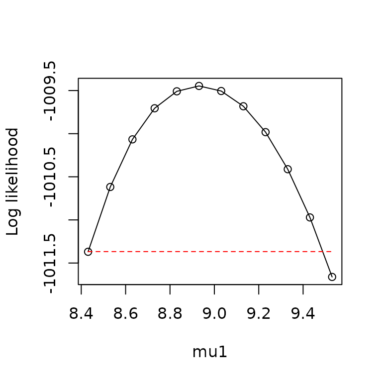

Note that the profiler stops its leftward (respectively, rightward) progress when num_steps_left (resp., num_steps_right) is exceeded, or when the threshold is crossed, whichever happens first. Profiling is often a trial-and-error process of selecting values for increment_left, increment_right, num_steps_left, and num_steps_right to get complete and smooth profiles within the limits of available computational resources.

Often one wants to plot the values of the other parameters which optimized the likelihood for each value of the profiled parameter. This can be done using the parameters output of profile_likelihood():

head(prof1$parameters)

##        mu1      mu2   sigltil1  sigltil2  sigrtil1   sigrtil2      ctil
## 1 8.430785 2.385404 -0.2362704 -1.672195 -1.761903 -0.5080501 -9.616414
## 2 8.530785 2.338315 -0.2196251 -1.602792 -1.796076 -0.5309846 -9.517754
## 3 8.630785 2.295559 -0.2024252 -1.535454 -1.829379 -0.5538060 -9.408728
## 4 8.730785 2.266397 -0.1872278 -1.467328 -1.851731 -0.5773561 -9.283236
## 5 8.830785 2.240172 -0.1712354 -1.401314 -1.874206 -0.6009431 -9.150693
## 6 8.930785 2.215594 -0.1542254 -1.337747 -1.898330 -0.6245366 -9.014500
##         pd    o_par1
## 1 2.032593 -1.458201
## 2 2.035249 -1.435857
## 3 2.038067 -1.413966
## 4 2.040938 -1.392952
## 5 2.043956 -1.371919
## 6 2.046990 -1.350736

pairs(prof1$parameters)

As a reminder, these are math-scale parameters.

Finally, the found_better output of profile_likelihood() is a flag which tells you whether, in the course of profiling, a higher likelihood was found than what was previously believed to be the maximum likelihood:

prof1$found_better

## [1] FALSE

In this case, a better value was not found, which provides additional evidence that we had previously already succeeded in adequately maximizing the likelihood. If found_better is TRUE, it means you have to go back and re-optimize, either with more initial conditions, or with tighter tolerances on the optimizer used, or with a different optimizer. Although sometimes it can be sufficient to simply re-start profiling using the parameters which were found via the first profiling effort to yield a new highest likelihood.

We next produce and plot all the profiles for our AIC-best model, where now the profiles are going to be plotted on the biological scale. Since the data are for a virtual species, they were generated with known true parameters. We also plot the true parameter values together with the profiles, to verify that the fitting process has accurately recovered the true parameters. This exercise is complicated by the redundancy, discussed above, of parameters. See below for details of how to resolve that redundancy. First make the profiles:

pnames <- names(make_mask_names(2))
all_profiles <- list()
for (counter in 1:length(pnames))
{
  all_profiles[[counter]] <- profile_likelihood(
                              profile_parameter=pnames[counter],
                              increment_left=0.05,
                              increment_right=0.05,
                              num_steps_left=50,
                              num_steps_right=50,
                              alpha=0.95,
                              optim_param_vector=all_optim_results[[1]]$par,
                              env_dat=env_array,
                              occ=occ,
                              num_threads=6
                            )
}
names(all_profiles) <- pnames

Now, to deal with the parameter redundancy, convert the maximum-likelihood parameters to the biological scale and find the representation of the true parameters which is closest in parameter space to the maximum-likelihood parameters:

example_1_true_parameters_bio <- example_1$true_par_list
example_1_true_parameters_bio

## $mu
## [1] 9.0 2.5
## 
## $sigltil
## [1] 0.3 0.2
## 
## $sigrtil
## [1] 0.5 0.8
## 
## $ctil
## [1] -9
## 
## $pd
## [1] 0.8649783
## 
## $o_mat
##           [,1]       [,2]
## [1,] 0.9800666 -0.1986693
## [2,] 0.1986693  0.9800666

ML_parameters_bio <- math_to_bio(all_optim_results[[1]]$par)
example_1_true_parameters_bio<-
  dist_between_params(example_1_true_parameters_bio,
                                    ML_parameters_bio,
                                    give_closest_rep=TRUE)$representative
example_1_true_parameters_bio

## $mu
## [1] 9.0 2.5
## 
## $sigltil
## [1] 0.8 0.3
## 
## $sigrtil
## [1] 0.2 0.5
## 
## $ctil
## [1] -9
## 
## $pd
## [1] 0.8649783
## 
## $o_mat
##            [,1]      [,2]
## [1,]  0.1986693 0.9800666
## [2,] -0.9800666 0.1986693

Now plot profiles. Recall we are plotting on the biological scale, so each parameter is transformed before the profile is plotted:

par(mfrow=c(3,3))

plot_tool <- function(x,y,thresh,xlab,true_param)
{
  plot(x,y,type="o",xlab=xlab,ylab="Log likelihood")
  lines(range(x),rep(thresh,2),type="l",
        lty="dashed",col="red")
  points(true_param,thresh,
        col="red",pch=20,cex=2)
}

#mu1
plot_tool(x = all_profiles$mu1$profile$value_math,
  y = all_profiles$mu1$profile$loglik,
  thresh = all_profiles$mu1$threshold,
  xlab = "mu1",
  true_param = example_1_true_parameters_bio$mu[1])

#mu2
plot_tool(x = all_profiles$mu2$profile$value_math,
  y = all_profiles$mu2$profile$loglik,
  thresh = all_profiles$mu2$threshold,
  xlab = "mu2",
  true_param = example_1_true_parameters_bio$mu[2])

#sigltil1 - need to exp transform to get to the bio scale
plot_tool(x = exp(all_profiles$sigltil1$profile$value_math),
  y = all_profiles$sigltil1$profile$loglik,
  thresh = all_profiles$sigltil1$threshold,
  xlab = "sigltil1",
  true_param = example_1_true_parameters_bio$sigltil[1])

#sigltil2 - need to exp transform to get to the bio scale
plot_tool(x = exp(all_profiles$sigltil2$profile$value_math),
  y = all_profiles$sigltil2$profile$loglik,
  thresh = all_profiles$sigltil2$threshold,
  xlab = "sigltil2",
  true_param = example_1_true_parameters_bio$sigltil[2])

#sigrtil1 - need to exp transform to get to the bio scale
plot_tool(x = exp(all_profiles$sigrtil1$profile$value_math),
  y = all_profiles$sigrtil1$profile$loglik,
  thresh = all_profiles$sigrtil1$threshold,
  xlab = "sigrtil1",
  true_param = example_1_true_parameters_bio$sigrtil[1])

#sigrtil2 - need to exp transform to get to the bio scale
plot_tool(x = exp(all_profiles$sigrtil2$profile$value_math),
  y = all_profiles$sigrtil2$profile$loglik,
  thresh = all_profiles$sigrtil2$threshold,
  xlab = "sigrtil2",
  true_param = example_1_true_parameters_bio$sigrtil[2])

#ctil
plot_tool(x = all_profiles$ctil$profile$value_math,
  y = all_profiles$ctil$profile$loglik,
  thresh = all_profiles$ctil$threshold,
  xlab = "ctil",
  true_param = example_1_true_parameters_bio$ctil)

#pd - need to expit transform to get to the bio scale
plot_tool(x = expit(all_profiles$pd$profile$value_math),
  y = all_profiles$pd$profile$loglik,
  thresh = all_profiles$pd$threshold,
  xlab = "pd",
  true_param = example_1_true_parameters_bio$pd)

#o_mat - Note that this is a single parameter on the math scale, so we only
#need to profile one of the matrix entries on the biological scale
x <- sapply(X=all_profiles$o_par1$profile$value_math,
           FUN=function(x){build_orthogonal_matrix(x)[1,1]})
plot_tool(x = x,
  y = all_profiles$o_par1$profile$loglik,
  thresh = all_profiles$o_par1$threshold,
  xlab = "o_par1",
  true_param = example_1_true_parameters_bio$o_mat[1,1])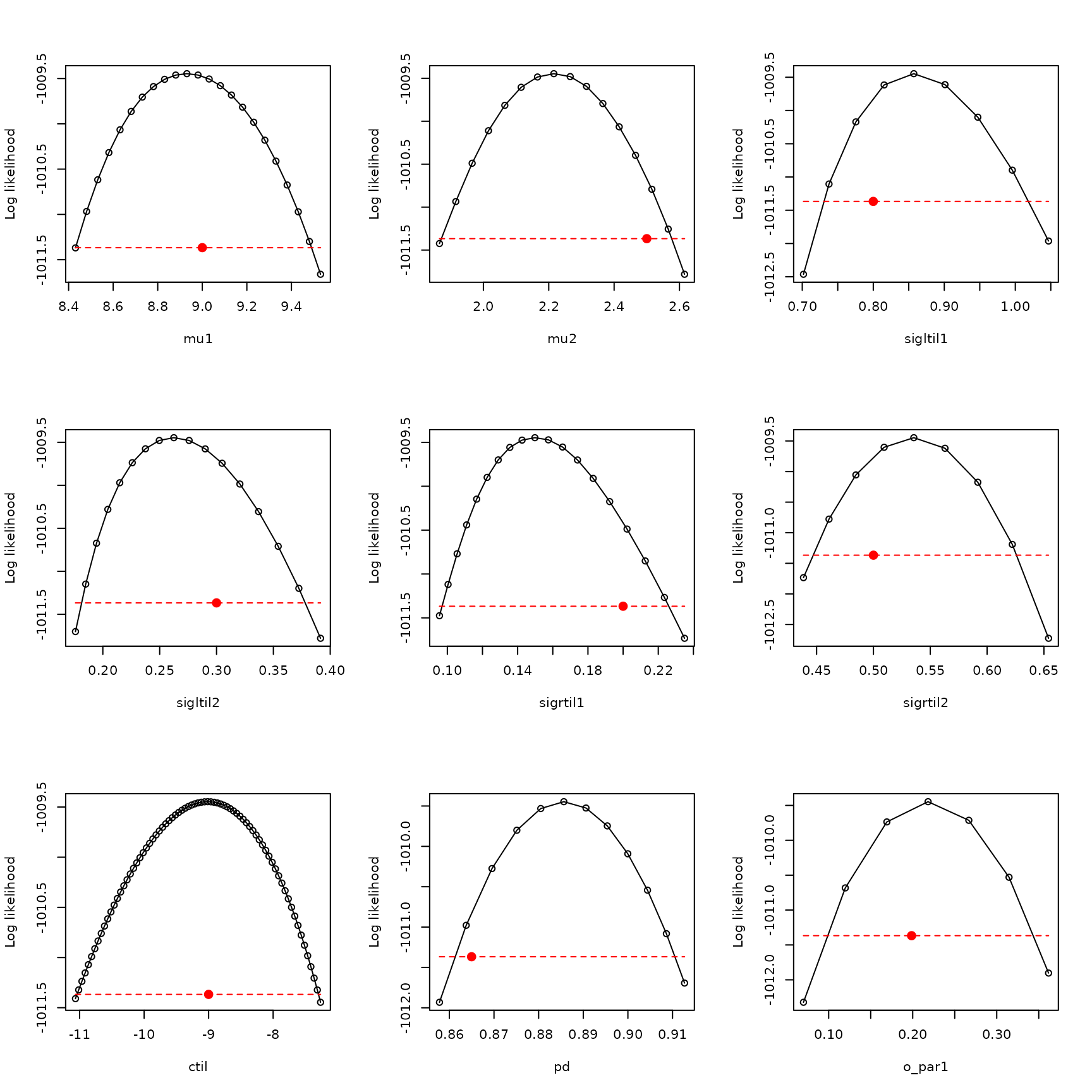

Note that transforming o_par profiles to the biological scale will not work the same way for more than two environmental variables because, in that case, there are multiple o_par parameters, and they interact with each other in the transformation to the biological scale. In that case, a Bayesian approach may have advantages.

Habitat suitability maps

We have now fitted several models, selected a best one, verified that the profiles look good, and shown that fitting captures the true model parameters. Habitat suitability maps are done with the habitat_suitability() function.

#plot the habitat suitability map
par(mfrow=c(2,3))
hab_suit <- habitat_suitability(param_list=ML_parameters_bio, env_list=env_data)
terra::plot(hab_suit,main="Habitat suitability",xlab="x",ylab="y",legend=TRUE)

#plot the true habitat suitability map
hab_suit_true <- habitat_suitability(param_list=example_1_true_parameters_bio, env_list=env_data)
terra::plot(hab_suit_true,main="Habitat suitability, true",
            xlab="x",ylab="y",legend=TRUE)

#plot the difference
terra::plot(hab_suit-hab_suit_true,main="Difference",
            xlab="x",ylab="y",legend=TRUE)

#plot the species ranges assuming a threshold of 0.5
terra::plot((hab_suit>.5),main="Species range",
            xlab="x",ylab="y",legend=TRUE)
terra::plot((hab_suit_true>.5),main="Species range, true",
            xlab="x",ylab="y",legend=TRUE)

#plot the difference
terra::plot((hab_suit>.5)-(hab_suit_true>.5),
            main="Difference",
            xlab="x",ylab="y",legend=TRUE)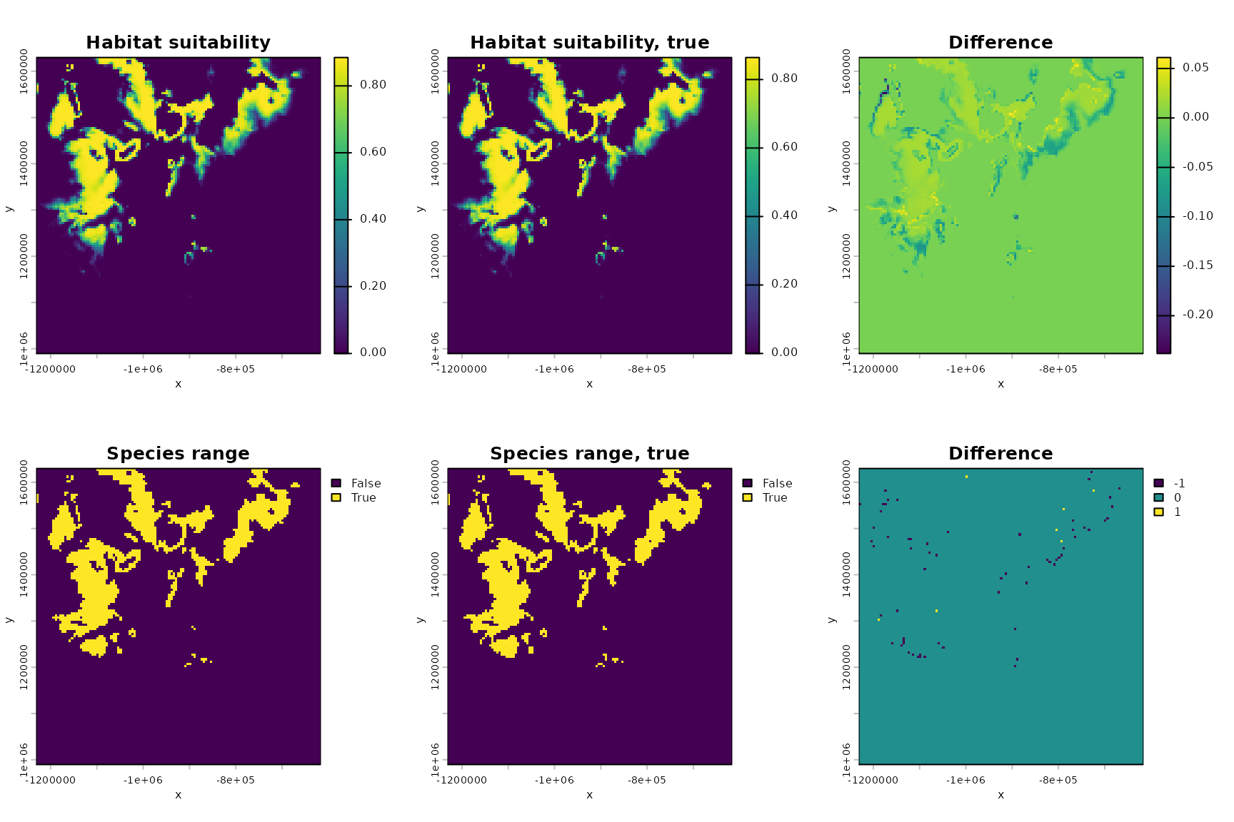

#compute percent error in range
area <- sum(as.data.frame((hab_suit_true>.5)))
area_setdiff <- sum(abs(as.data.frame((hab_suit>.5)-(hab_suit_true>.5))-0)>1e-1)
delta <- (area_setdiff)/area
area

## [1] 2058

area_setdiff

## [1] 69

delta

## [1] 0.0335277

As you can see, both the inferred habitat suitability map and the associated species range are similar to the true versions.

One of the main things xsdm is good for is assessing the influence of inter-annual climatic variability on species distributions, so we also display what the habitat suitability map would look like if the value of each environmental variable in each location were always equal to the temporal mean for that variable and location. We use inferred parameters.

#plot the habitat suitability map again, to ease comparisons
par(mfrow=c(2,3))
hab_suit <- habitat_suitability(param_list=ML_parameters_bio, env_list=env_data)
terra::plot(hab_suit,main="Habitat suitability",xlab="x",ylab="y",legend=TRUE)

#plot the habitat suitability map without variability
m_bio_1_ts <- rep(m_bio_1,terra::nlyr(bio_1))
m_bio_12_ts <- rep(m_bio_12,terra::nlyr(bio_12))
m_env_data <- list(m_bio_1=m_bio_1_ts,m_bio_12=m_bio_12_ts)
m_hab_suit <- habitat_suitability(param_list=ML_parameters_bio, env_list=m_env_data)
terra::plot(m_hab_suit,main="Habitat suitability, no var",
            xlab="x",ylab="y",legend=TRUE)

#plot the difference
terra::plot(m_hab_suit-hab_suit,main="Difference",
            xlab="x",ylab="y",legend=TRUE)

#plot the species ranges assuming a threshold of 0.5
terra::plot((hab_suit>.5),main="Species range",
            xlab="x",ylab="y",legend=TRUE)
terra::plot((m_hab_suit>.5),main="Species range, no var",
            xlab="x",ylab="y",legend=TRUE)

#plot the difference
terra::plot((m_hab_suit>.5)-(hab_suit>.5),
            main="Difference",
            xlab="x",ylab="y",legend=TRUE)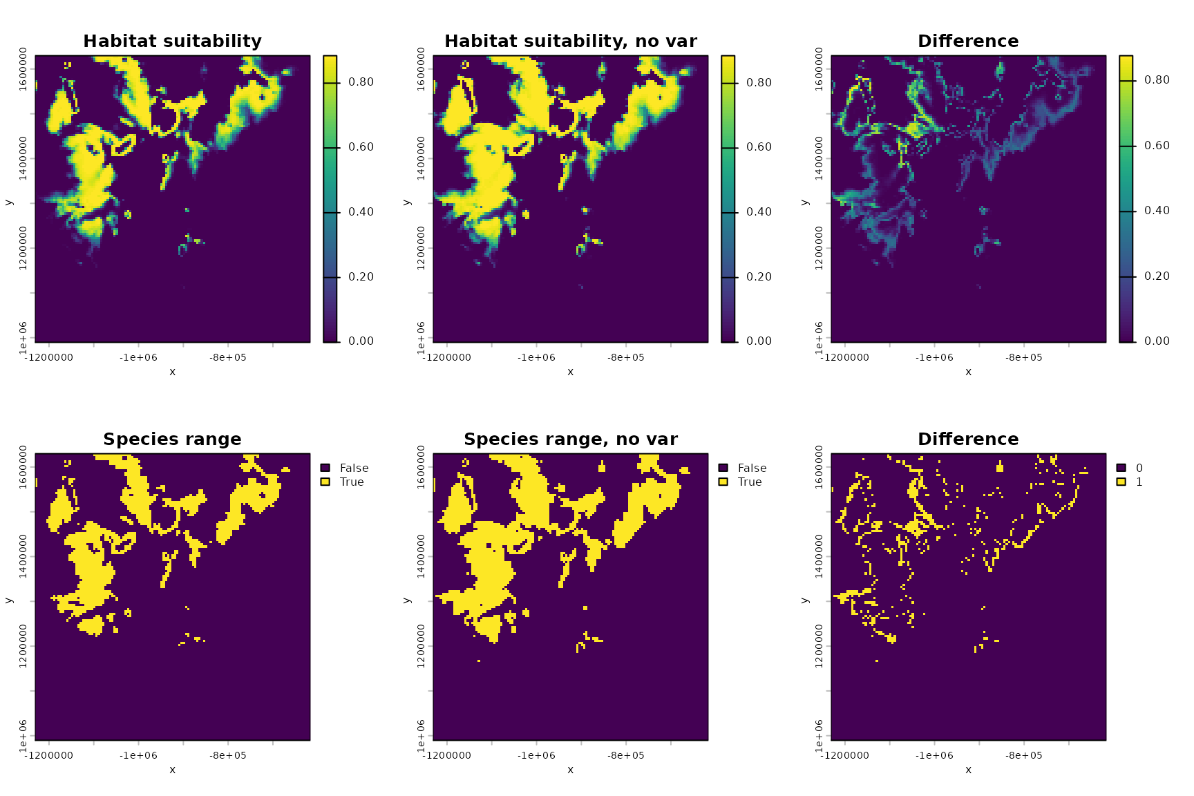

#compute change in area due to variability
area <- sum(as.data.frame((hab_suit>.5)))
area_novar <- sum(as.data.frame((m_hab_suit>.5)))
delta_area <- (area_novar-area)/area_novar
area

## [1] 2003

area_novar

## [1] 2716

delta_area

## [1] 0.2625184

So we see variability reduces area by a certain percentage for this virtual species.

Interpreting model parameters

We would like to interpret the the parameters of the fitted model to say what we can about how the species responds to the environment. This is rendered a bit more challenging due to the parameter reduction step which was carried out for the model to eliminate structural non-identifiability (see “The xsdm statistical model” for details). The function interpret_parameters() helps with this, displaying plots which describe the inferred growth-environment function (the relationship between the environment, \(\vec{e}_t\), in a given year in a location and the annual net growth rate, \(\lambda_t\)). For instance, for our example, the contours of that function are determined, though their heights are not determined. The contours are enough to tell the user what the optimal environment is for the species, and how sensitive annual net growth is to departures from this optimum for each environmental variable, relative to the other environmental variables:

par(mfrow=c(1,2))
interpret_parameters(param_list=ML_parameters_bio,
                     plot_indices=c(1,2),
                     plot_lims=list(c(-9.5,13),c(-5.5,17)))
title(main="Inferred")
points(env_array[occ==1,,1],env_array[occ==1,,2],pch=20,
       col=rgb(0,0,0,.2),cex=0.2)

interpret_parameters(param_list=ML_parameters_bio,
                     plot_indices=c(1,2),
                     plot_lims=list(c(-9.5,13),c(-5.5,17)))
title(main="Inferred")
points(env_array[occ==0,,1],env_array[occ==0,,2],pch=20,
       col=rgb(0,0,0,.2),cex=0.2)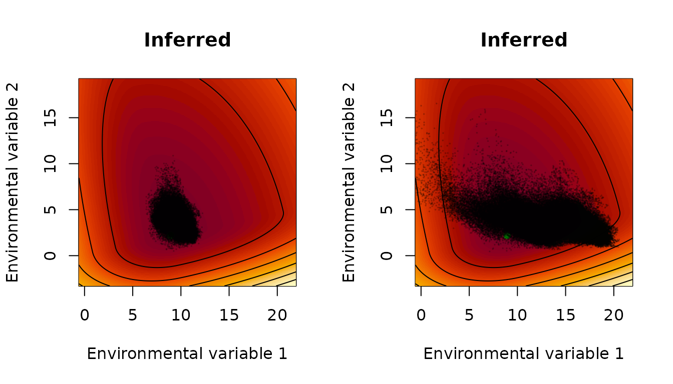

The points displayed here are all values of the environmental variables, in any year, in locations for which the species was detected (left) or assumed absent (right). One can see that growth is inferred to be more sensitive to low temperatures (leftward departures of environmental variable 1 from the optimum) than it is to high temperatures (rightward departures); and growth is more sensitive to drought (downward departures of environmental variable 2 from the optimum) than it is to abundant rainfall (upward departures). One can see that, as expected, the environment is more suitable for population growth, according to the inferred growth-environment function, in locations in which the species was observed. One can see that, even in locations found to be unsuitable for the species (right panel), there were plenty of individual years for which environmental conditions promoted growth in that year, demonstrating the importance of interannual variability.

Now we plot the same thing for the true parameters:

par(mfrow=c(1,2))
interpret_parameters(param_list=example_1_true_parameters_bio,
                     plot_indices=c(1,2),
                     plot_lims=list(c(-9.5,13),c(-5.5,17)))
title(main="True")
points(env_array[occ==1,,1],env_array[occ==1,,2],pch=20,
       col=rgb(0,0,0,.2),cex=0.2)

interpret_parameters(param_list=example_1_true_parameters_bio,
                     plot_indices=c(1,2),
                     plot_lims=list(c(-9.5,13),c(-5.5,17)))
title(main="True")
points(env_array[occ==0,,1],env_array[occ==0,,2],pch=20,
       col=rgb(0,0,0,.2),cex=0.2)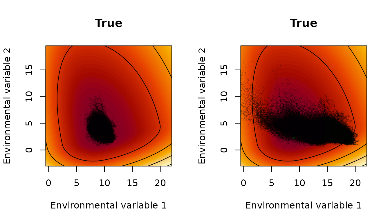

Results are quite similar. Plots against one environmental variable are also possible, holding the other one at optimal values. See the documentation of interpret_parameters() for details.

Daniel C. Reuman

Angel Luís Robles Fernández