Tool to help interpret xsdm model parameters — interpret

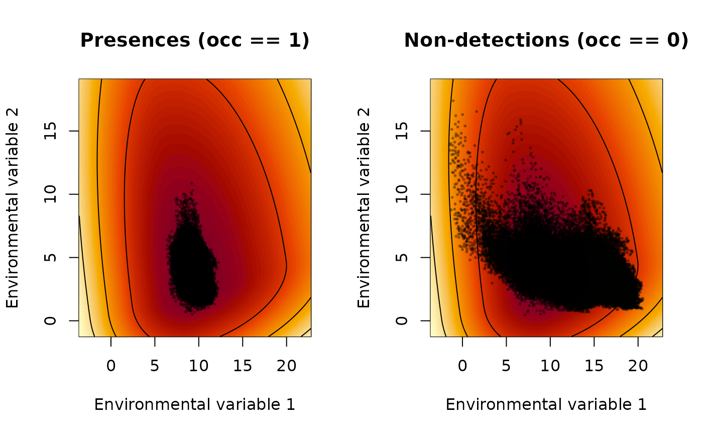
Due to the parameter reduction step which was carried out to eliminate structural non-identifiability in the xsdm model, parameter interpretation is more difficult. This function helps with that difficulty, displaying contours for the inferred log growth-environment function. The shapes of these contours are determined by inference, even though their levels are not; and the shapes are generally more informative anyway. See the manual documents “The xsdm model” and “How to fit xsdm models with species occurrence data using xsdm” for additional details.

Usage

interpret_parameters(
  param_list,
  plot_indices,
  plot_lims = NULL,
  env_dat = NULL,
  occ = NULL,
  breadth = 1,
  ...
)

Arguments

param_list: A named list of xsdm model parameters such as returned by math_to_bio. Must contain elements mu, sigltil, sigrtil, ctil, pd, and o_mat.
plot_indices: A length-1 or length-2 integer vector of indices of environmental variables against which the growth-environment function is to be plotted. For a length-2 vector, the first index is the horizontal axis, the second the vertical. Other environmental variables are held at their values in param_list$mu.
plot_lims: Optional list of the same length as plot_indices, each element a 2-vector giving the plotting extent *relative to* mu. If NULL (the default) and env_dat is supplied, limits are auto-derived via auto_plot_lims_() using the breadth argument. The auto-derived limits cover the full observed environmental range plus a symmetric margin on each side.
env_dat: Optional 3D numeric array of environmental data with dimensions (locations) x (time) x (variables). Required for the two-panel (presence vs non-detection) display and for auto-derived plot_lims. If NULL, a single-panel legacy plot is drawn and plot_lims must be supplied.
occ: Optional length-(locations) logical or 0/1 vector of presence/absence. Required together with env_dat for the two-panel display.
breadth: Scalar in [0, 1] controlling how wide the auto-derived plotting window is around mu: breadth = 1 (default) shows the full min-max environmental range plus a 10% margin on each side; breadth = 0 collapses to essentially a single point. Ignored when plot_lims is supplied.
...: Additional graphical arguments passed to plot (1D case) or image (2D case).

Value

Invisibly returns the (possibly auto-derived) plot_lims list, so downstream code can reuse the same limits. The main purpose of the function is its side effect: plots are sent to the default graphics device.

Details

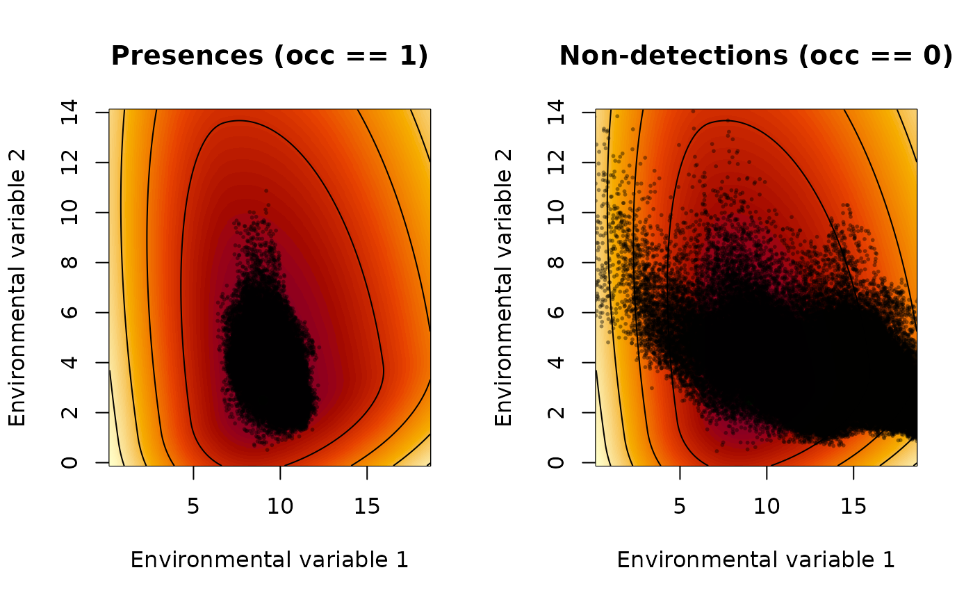
If env_dat and occ are provided, two panels are drawn side by side: on the left the growth-environment function is shown together with the environmental values at presence locations (occ == 1); on the right the same function is shown together with the environmental values at non-detections (occ == 0). Both panels share identical contour breaks (bivariate case) or identical axes (univariate case), so the two are directly comparable.

The log growth-environment function is determined by inference only up to an affine transformation $g = a f(e) + b$ with $a > 0$. Its contours are therefore unlabelled in the output; their shape is what is interpretively meaningful. In code the function is $$y(e) = -\sum_i \left( \frac{[u_i]_+}{\sigma^R_i} + \frac{[u_i]_-}{\sigma^L_i} \right)^2 , \quad u = O^{T} (e - \mu),$$ which is always $\le 0$, attains its maximum 0 at $e = \mu$, and decreases without bound as $e$ moves away from $\mu$. Consequently the numeric values on the y-axis of the univariate plot and the numeric values of the image colors in the bivariate plot carry no units of their own.

Examples

if (FALSE) { # \dontrun{
  # Two-panel (presence vs non-detection) plot with auto-derived limits
  interpret_parameters(
    example_1$par_list,
    plot_indices = c(1, 2),
    env_dat      = example_1$env_array,
    occ          = example_1$occ_vec
  )

  # Narrower auto-derived window
  interpret_parameters(
    example_1$par_list,
    plot_indices = c(1, 2),
    env_dat      = example_1$env_array,
    occ          = example_1$occ_vec,
    breadth      = 0.7
  )

} # }