Unusable models: when a model does not have a maximum likelihood

\[ \newcommand{\mean}[1]{\overline{#1}} \newcommand{\var}{\text{var}} \newcommand{\cov}{\text{cov}} \newcommand{\cor}{\text{cor}} \newcommand{\Rp}{\text{Re}} \newcommand{\E}{\text{E}} \newcommand{\ltsgr}{\text{ltsgr}} \newcommand{\expit}{\text{expit}} \newcommand{\logit}{\text{logit}} \]

Abstract. When an xsdm model does not have a maximum likelihood, it should not be used. This document shows an example of how that can occur, and how to diagnose it. Along the way, another type of boundary model (in addition to the \(p_d=1\) case described elsewhere) is illustrated. In the new boundary model, sigma parameters are set to infinity, corresponding to insensitivity of annual net growth to environmental changes in a certain direction in environment space. This example is based on occurrence data from GBIF for Ophisaurus ventralis, the Eastern glass lizard.

The Eastern glass lizard, Ophisaurus ventralis, is a legless lizard found in the southeastern United States. It is the longest and heaviest species of its genus, growing up to 108cm in total length.

We start by loading the data:

library(xsdm)
env_array <-  example_2$env_array

dim(env_array)

## [1] 2728   39    6

dimnames(env_array)[[3]]

## [1] "BIO01" "BIO10" "BIO11" "BIO12" "BIO16" "BIO17"

occ <-  example_2$occ_vec
length(occ)

## [1] 2728

Here, there are 6 environmental variables recorded for 39 years in 2728 locations, with accompanying detections and pseudo-absences in the variable occ. The first three environmental variables (BIO1, BIO10, BIO11) are temperature variables, and the last three (BIO12, BIO16, BIO17) are precipitation variables. BIO1 is mean annual temperature, BIO10 is mean temperature of the warmest quarter, BIO11 is mean temperature of the coldest quarter, BIO12 is annual precipitation, BIO16 is precipitation of the wettest quarter, and BIO17 is precipitation of the driest quarter.

Now look at the distributions of values of environmental variables to make sure they are not on very different scales, which could cause problems for optimization:

apply(FUN=quantile, X=env_array, MARGIN=3,prob=c(.025,.25,.5,.75,.975))

##       BIO01 BIO10 BIO11  BIO12 BIO16 BIO17
## 2.5%  12.21 21.39  3.85  88.08 10.14  2.21
## 25%   16.88 25.77  8.88 114.44 14.34  4.37
## 50%   18.71 26.64 11.53 131.58 17.40  5.78
## 75%   20.43 27.33 14.38 151.16 20.91  7.22
## 97.5% 24.30 28.30 20.73 195.81 29.55 10.72

These distributions look basically OK.

Now fit 15 models, each from 25 starting conditions:

models <- matrix(c(1,0,0,0,0,0,
                  0,1,0,0,0,0,
                  0,0,1,0,0,0,
                  0,0,0,1,0,0,
                  0,0,0,0,1,0,
                  0,0,0,0,0,1,
                  1,0,0,1,0,0,
                  1,0,0,0,1,0,
                  1,0,0,0,0,1,
                  0,1,0,1,0,0,
                  0,1,0,0,1,0,
                  0,1,0,0,0,1,
                  0,0,1,1,0,0,
                  0,0,1,0,1,0,
                  0,0,1,0,0,1), nrow=15, byrow=TRUE)
all_model_results <- list()
for (i in 1:nrow(models))
{
  env_dat <-  env_array[ , , models[i,]==1, drop = FALSE]
  starts <-  start_parms(env_dat[occ==1,,,drop=FALSE],num_starts=25)
  all_optim_results <-  list()
  for (j in 1:nrow(starts))
  {
    all_optim_results[[j]] <-  optim(par = starts[j,],
                                   fn = loglik_math,
                                   method = "BFGS",
                                   env_dat = env_dat,
                                   occ = occ,
                                   negative=TRUE,
                                   control = list(trace=0)
                                   )
  }
  all_model_results[[i]] <- all_optim_results
}

Within each model, rank the optimization results:

for (i in 1:length(all_model_results))
{
  values <-  sapply(X = all_model_results[[i]], FUN=function(x){x$value})
  inds <-  order(values)
  all_model_results[[i]] <-  all_model_results[[i]][inds]
}

Rank the models by BIC, bearing in mind that we’ve been working with the negative of the likelihood:

model_BICs <- sapply(X=all_model_results,
                      FUN=function(x){
                        best_loglik = x[[1]]$value
                        num_parms = length(x[[1]]$par)
                        n = length(occ)
                        BIC = 2*best_loglik + num_parms*log(n)
                        return(BIC)
                      }
                    )

Also by AIC, then display:

model_AICs <- sapply(X=all_model_results,
                      FUN=function(x){
                        best_loglik = x[[1]]$value
                        num_parms = length(x[[1]]$par)
                        AIC = 2*best_loglik + 2*num_parms
                        return(AIC)
                      }
                    )

inds <- order(model_BICs)
rbind(model_BICs[inds],model_AICs[inds])

##          [,1]     [,2]     [,3]     [,4]     [,5]     [,6]     [,7]     [,8]
## [1,] 2419.993 2473.974 2482.634 2550.379 2580.207 2586.112 2593.000 2593.550
## [2,] 2366.792 2420.772 2429.433 2520.822 2550.650 2556.556 2539.799 2540.348
##          [,9]    [,10]    [,11]    [,12]    [,13]    [,14]    [,15]
## [1,] 2594.320 2595.875 2602.761 2676.556 2682.887 2915.417 2945.898
## [2,] 2541.118 2542.673 2549.560 2647.000 2629.686 2885.860 2916.341

plot(model_BICs,model_AICs,type="p",xlab="BIC",ylab="AIC")

order(model_BICs)

##  [1] 11  8 14  5  3  1  7 13  9 15 10  2 12  4  6

order(model_AICs)

##  [1] 11  8 14  5  7 13  9 15 10  3  1 12  2  4  6

The AIC and BIC results are pretty well aligned, and the four best models are the same:

models[order(model_BICs)[1:4],]

##      [,1] [,2] [,3] [,4] [,5] [,6]
## [1,]    0    1    0    0    1    0
## [2,]    1    0    0    0    1    0
## [3,]    0    0    1    0    1    0
## [4,]    0    0    0    0    1    0

These four models all use the same predictor, the fifth one, and then some use various possible second predictors.

We emphasize that these BIC and AIC values may or may not be meaningful, since B/AIC can only be computed when the likelihood has been effectively maximized. We will elaborate below, but for now we accept these are pseudo-BIC and pseudo-AIC values, subject to later validation or rejection.

Among the models we fitted, there is one clear winner in pseudo-BIC (the model with the lowest pseudo-BIC). So let’s investigate it further. Start by optimizing it a bit harder to see if we can do any better.

i <- 11
env_dat <- env_array[,,models[i,]==1,drop=FALSE]
starts <- start_parms(env_dat[occ==1,,,drop=FALSE], num_starts = 100)
model_11_results <- list()
for (j in 1:nrow(starts))
{
  model_11_results[[j]] <- optim(par=starts[j,],fn=loglik_math,
                                method="BFGS",
                                env_dat = env_dat,
                                occ = occ,negative=TRUE,
                                control = list(trace=0))
}
all_model_results[[11]][[1]]$value

## [1] 1174.396

min(sapply(X=model_11_results, FUN=function(y){y$value}))

## [1] 1174.354

About the same.

Now move forward by looking at the results for this model, starting by writing a convenience function for examine optimization results:

examine_optim_results <- function(optim_results,mask=NULL)
{
  #put optimization results in order from best to worst
  bestlogliks <- sapply(X=optim_results,FUN=function(x){x$value})
  inds <- order(bestlogliks)
  bestlogliks <- bestlogliks[inds]
  optim_results <- optim_results[inds]

  #model convergence
  convergences <- sapply(X=optim_results,FUN=function(x){x$convergence})

  #compute distances to the best result in parameter space
  best_parms_math <- optim_results[[1]]$par
  parms_dists_to_best <- lapply(
    X=optim_results,
    FUN=function(x){
      dist_between_params(
        x$par,
        best_parms_math,
        mask=mask,
        give_closest_rep=TRUE)
    }
  )
  parms_dists <- sapply(X=parms_dists_to_best, FUN=function(x){x$distance})
  bestparms <- sapply(X=parms_dists_to_best, FUN=function(x){unlist(x$representative)})

  #put it all together
  return(rbind(bestlogliks,convergences,parms_dists,bestparms))
}

h <- examine_optim_results(all_model_results[[11]])
t(h[ ,1:8])

##      bestlogliks convergences parms_dists      mu1      mu2     sigltil1
## [1,]    1174.396            0    0.000000 29.53229 49.10733 6.312314e-01
## [2,]    1174.478            0    3.659640 29.31359 45.68728 6.324729e-01
## [3,]    1174.524            1    3.657095 29.28334 45.66600 6.431441e-01
## [4,]    1174.615            1    7.370553 29.07606 42.23728 6.384445e-01
## [5,]    1174.639            1    7.664594 29.06959 42.00460 6.535947e-01
## [6,]    1174.765            1    7.671312 29.02223 41.83031 6.206297e-01
## [7,]    1198.763            0   29.464908 24.98672 22.77742 3.202862e+04
## [8,]    1217.073            0   28.167206 40.95720 24.17343 3.734968e+02
##      sigltil2  sigrtil1   sigrtil2       ctil        pd     o_mat1      o_mat2
## [1,] 6.733026 0.3218009   13.85173 -13.278926 0.5393361  0.9965467 -0.08303475
## [2,] 6.388541 0.3232464 3339.36142 -11.997158 0.5417885  0.9963504 -0.08535778
## [3,] 6.351200 0.3212587  433.71436 -12.069050 0.5397711  0.9964882 -0.08373307
## [4,] 6.038240 0.3226673 3492.80325 -10.649592 0.5443655  0.9961846 -0.08727052
## [5,] 6.040673 0.3174715  204.19111 -10.437524 0.5461967  0.9962345 -0.08669963
## [6,] 5.887293 0.3307282   52.35843 -10.907681 0.5403760  0.9960977 -0.08825696
## [7,] 2.798811 0.1194403  179.82104  -2.325735 0.6155530 -0.9993029  0.03733265
## [8,] 4.202790 0.6395854   20.48267  -7.368288 0.5347857  0.6021973 -0.79834728
##          o_mat3    o_mat4
## [1,] 0.08303475 0.9965467
## [2,] 0.08535778 0.9963504
## [3,] 0.08373307 0.9964882
## [4,] 0.08727052 0.9961846
## [5,] 0.08669963 0.9962345
## [6,] 0.08825696 0.9960977
## [7,] 0.03733265 0.9993029
## [8,] 0.79834728 0.6021973

The very large values of sigrtil1 suggest the boundary model where this parameter is set to Inf, corresponding to a direction in environment space along which annual net growth is insensitive to changes in the environment.

So we consider the corresponding boundary model:

i <- 11
env_dat <- env_array[ , , models[i,] == 1, drop=FALSE]
mask <- c(sigrtil1 = Inf)
new_starts <- start_parms(env_dat[occ == 1, , , drop=FALSE],
                               mask = mask,
                               num_starts = 100)

bdry_optim_results <- list()
for (j in 1:nrow(new_starts))
{
  bdry_optim_results[[j]] <- optim(par = new_starts[j,],
                                  fn = loglik_math,
                                  method = "BFGS",
                                  env_dat = env_dat,
                                  occ = occ,
                                  mask = mask,
                                  negative = TRUE,
                                  control = list(trace=0, maxit=500))
}

Now look at these results:

h <- examine_optim_results(bdry_optim_results, mask = mask)
t(h[ ,1:8])

##      bestlogliks convergences parms_dists      mu1      mu2 sigltil1  sigltil2
## [1,]    1174.314            0    0.000000 29.80781 52.48489 7.077802 0.3178120
## [2,]    1174.347            0    2.664900 29.61165 50.05280 6.888541 0.3225889
## [3,]    1174.381            0    2.084646 29.61994 50.50126 6.856338 0.3205543
## [4,]    1174.393            0    4.670735 29.50979 48.19736 6.724723 0.3179098
## [5,]    1174.416            0    4.050722 29.48807 48.65409 6.672816 0.3282775
## [6,]    1174.427            0    6.168444 29.42779 46.73657 6.537189 0.3194078
## [7,]    1174.429            0    4.701824 29.44205 48.06048 6.623281 0.3220493
## [8,]    1174.429            0    3.846229 29.50345 48.82800 6.674206 0.3219386
##      sigrtil1  sigrtil2      ctil        pd     o_mat1    o_mat2     o_mat3
## [1,]      Inf 0.6393998 -14.44921 0.5393101 0.08238505 0.9966006 -0.9966006
## [2,]      Inf 0.6355975 -13.37877 0.5412292 0.08290388 0.9965575 -0.9965575
## [3,]      Inf 0.6335596 -13.83706 0.5385828 0.08206070 0.9966273 -0.9966273
## [4,]      Inf 0.6452119 -12.62062 0.5423834 0.08388754 0.9964752 -0.9964752
## [5,]      Inf 0.6204243 -13.17693 0.5391875 0.08366047 0.9964943 -0.9964943
## [6,]      Inf 0.6395714 -12.24428 0.5426578 0.08559728 0.9963298 -0.9963298
## [7,]      Inf 0.6320109 -12.90138 0.5396961 0.08292752 0.9965556 -0.9965556
## [8,]      Inf 0.6288177 -13.29787 0.5383230 0.08297769 0.9965514 -0.9965514
##          o_mat4
## [1,] 0.08238505
## [2,] 0.08290388
## [3,] 0.08206070
## [4,] 0.08388754
## [5,] 0.08366047
## [6,] 0.08559728
## [7,] 0.08292752
## [8,] 0.08297769

The best likelihoods obtained for this boundary model are very similar to those obtained for the initial, non-boundary model, and the boundary model has one fewer parameter, so we tentatively adopt the boundary model over the earlier model. However, these optimization results reveal that we probably still have not successfully optimized the likelihood, or that the likelihood surface may have a ridge or an asymptote or other pathological feature. One sees this by observing that whereas the top several optimization results are similar in likelihood, they are spread out in parameter space (the parms_dists column shows distance in parameter space to the top-likelihood result).

To investigate the model further, we profile:

pnames <-  names(make_mask_names(2))
pnames <-  pnames[!(pnames %in% names(mask))]

values <-  sapply(X=bdry_optim_results, FUN=function(x){x$value})
inds <-  order(values)
bdry_optim_results <-  bdry_optim_results[inds]

all_profiles <- list()
linc <-  rep(0.05, length(pnames))
rinc <-  rep(0.05, length(pnames))
linc[8] <-  0.001
rinc[8] <-  0.001
for (counter in 1:length(pnames))
{
  all_profiles[[counter]] <-  profile_likelihood(
                              profile_parameter = pnames[counter],
                              increment_left =linc[counter],
                              increment_right = rinc[counter],
                              num_steps_left = 50,
                              num_steps_right = 50,
                              alpha = 0.95,
                              optim_param_vector = bdry_optim_results[[1]]$par,
                              env_dat=env_dat,
                              occ = occ,
                              mask = mask,
                              num_threads = 6
                            )
}
names(all_profiles) <-  pnames

Now plot these profiles:

plot_tool <- function(ap,index)
  {
  x <- ap[[index]]$profile$value_math
  y <- ap[[index]]$profile$loglik
  xlab <- names(ap)[index]
  thresh <- ap[[index]]$threshold
  plot(x,y,
       type="o",xlab=xlab,
       ylab="Log likelihood")
  lines(range(x),rep(thresh,2),type="l",
        lty="dashed",col="red")
}

par(mfrow=c(3,3))
plot_tool(all_profiles, 1)
plot_tool(all_profiles, 2)
plot_tool(all_profiles, 3)
plot_tool(all_profiles, 4)
plot_tool(all_profiles, 5)
plot_tool(all_profiles, 6)
plot_tool(all_profiles, 7)
plot_tool(all_profiles, 8)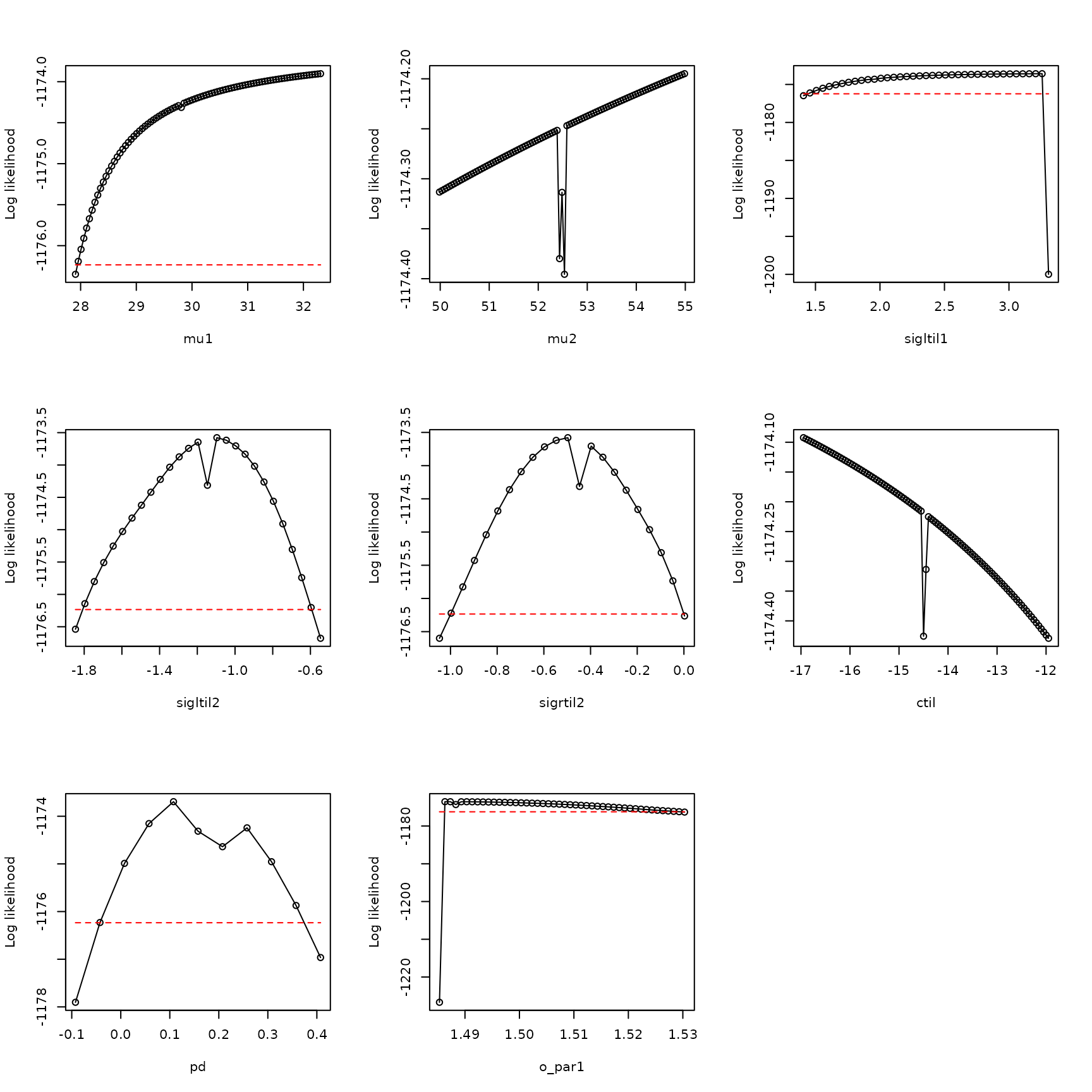

These profiles are not dome-shaped, and have other idiosyncratic features, confirming that we had not effectively optimized the likelihood. The mu1, mu2, and ctil profiles, in particular, show problems. These results suggest a ridge in the likelihood surface that may rise asymptotically along some path in parameter space for which mu2 is increasing. We have not identified a maximum of the likelihood function, and it looks as though there may not be one if the increase is indeed asymptotic.

We look at what the growth-environment function looks like for the best parameters we have found so far, maybe that will give some insight into what is going wrong:

param_list <- bdry_optim_results[[1]]$par
param_list["sigrtil1"] <- Inf
param_list <- param_list[names(make_mask_names(2))]
param_list_bio <- math_to_bio(param_list)
interpret_parameters(param_list = param_list_bio,
                          plot_indices = c(1,2), env_dat=env_dat, occ = occ)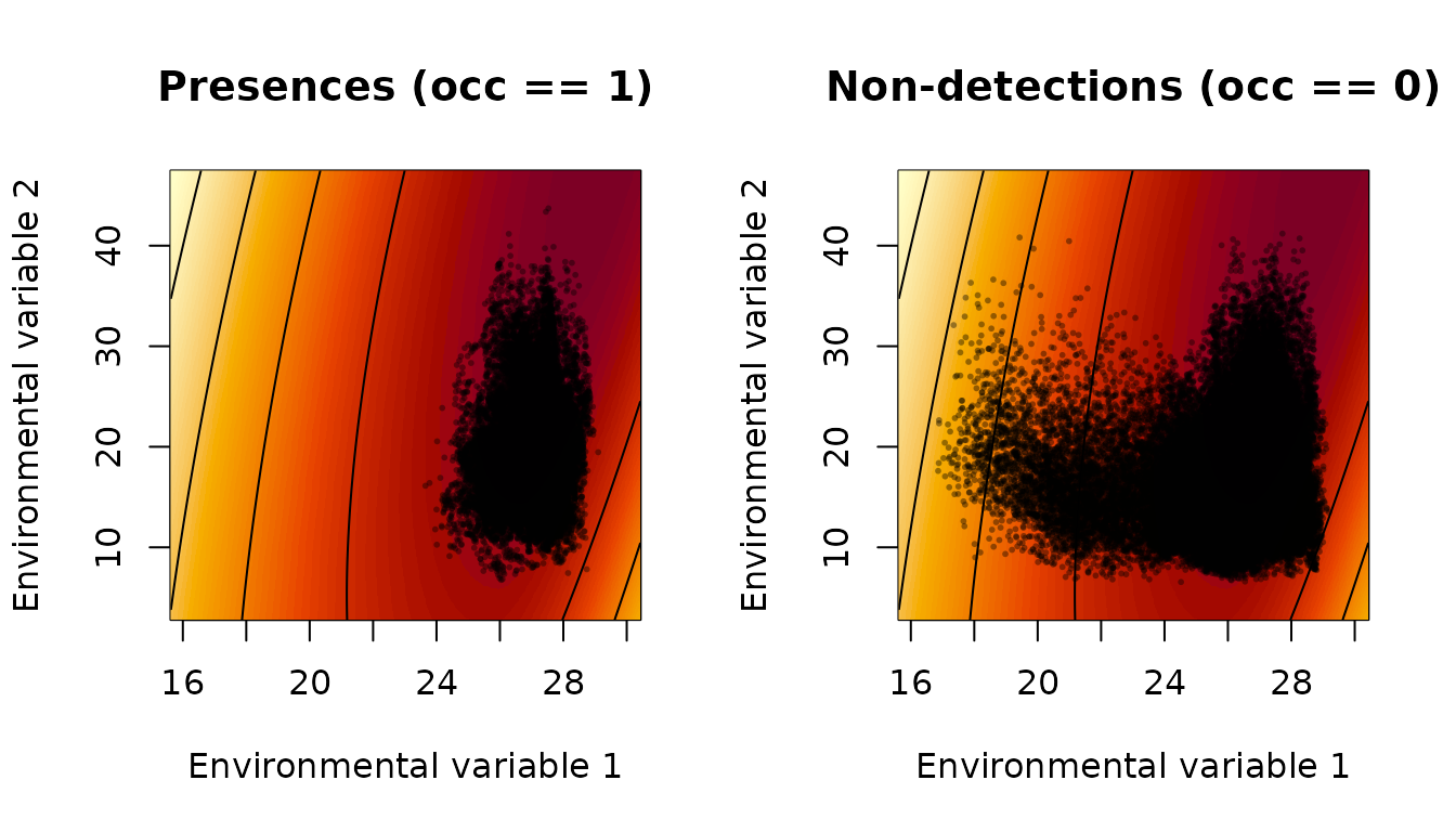

param_list_bio$mu

## [1] 29.80781 52.48489

Estimated values of mu2 are outside the range of the environmental data. The actual distribution of the species is across Florida and along the coasts of the Southeastern United States, and the southern extent of the species is very likely constrained, on the southern end of the range, by the Atlantic Ocean and the Gulf of Mexico rather than by temperature and precipitation. Ultimately the modeling probably fails here for these reasons. A Bayesian approach to the same problem could likely address some of the limitations, here, by setting appropriate priors. In the frequentist setting, one must discard the model. AIC and BIC values are invalid when the likelihood has not been adequately optimized and when the likelihood surface in the vicinity of the optimum is not approximately a dome.

Immediate next steps should include examination of the second- and third-best models according to pseudo-BIC, to see if they have similar problems. For brevity and because we are just trying to illustrate statistical principles and workflows, we skip straight to examining the fourth-best model, which may be simpler because it only uses one environmental variable.

i <- 5
model_5_optim_results <-  all_model_results[[i]]
h <- examine_optim_results(model_5_optim_results)
t(h[,1:8])

##      bestlogliks convergences  parms_dists       mu  sigltil      sigrtil
## [1,]    1255.411            0 0.0000000000 21.33012 2.399187 1208873.3242
## [2,]    1255.411            0 0.0001590943 21.33012 2.399232 1072536.0598
## [3,]    1255.411            0 0.0002968734 21.32996 2.399115 5999992.9188
## [4,]    1255.411            0 0.0008332980 21.32946 2.398987    1943.3197
## [5,]    1255.411            0 0.0011494547 21.32968 2.399102     959.3546
## [6,]    1255.411            0 0.0012001110 21.33004 2.399171     834.9980
## [7,]    1255.411            0 0.0028224249 21.33003 2.399168     354.4335
## [8,]    1255.412            0 0.0056786477 21.33120 2.399464     179.8249
##           ctil        pd o_mat
## [1,] -1.806488 0.6390043     1
## [2,] -1.806330 0.6390243     1
## [3,] -1.806742 0.6389815     1
## [4,] -1.806512 0.6389836     1
## [5,] -1.806276 0.6390270     1
## [6,] -1.806444 0.6390100     1
## [7,] -1.806433 0.6390213     1
## [8,] -1.806874 0.6389664     1

One can see the boundary model with sigrtil set to Inf should be considered:

env_dat <- env_array[,,models[i,]==1,drop=FALSE]
mask <- c(sigrtil1 = Inf)
new_starts <- start_parms(env_dat[occ==1,,,drop=FALSE],mask=mask,
                               num_starts=100)

bdry_optim_results5 <- list()
for (j in 1:nrow(new_starts))
{
  bdry_optim_results5[[j]] <- optim(par=new_starts[j,],fn=loglik_math,
                                method="BFGS",
                                env_dat=env_dat,occ=occ,mask=mask,negative=TRUE,
                                control=list(trace=0,maxit=500))
}

Examine these results:

h <- examine_optim_results(bdry_optim_results5,mask=mask)
t(h[,1:8])

##      bestlogliks convergences  parms_dists       mu  sigltil sigrtil      ctil
## [1,]    1255.411            0 0.000000e+00 21.32997 2.399159     Inf -1.806409
## [2,]    1255.411            0 9.275730e-05 21.33001 2.399151     Inf -1.806489
## [3,]    1255.411            0 6.953356e-05 21.32991 2.399151     Inf -1.806378
## [4,]    1255.411            0 8.098549e-05 21.33004 2.399171     Inf -1.806450
## [5,]    1255.411            0 5.519872e-05 21.33002 2.399175     Inf -1.806414
## [6,]    1255.411            0 6.522924e-05 21.33003 2.399177     Inf -1.806421
## [7,]    1255.411            0 5.004263e-05 21.32994 2.399167     Inf -1.806365
## [8,]    1255.411            0 7.438182e-05 21.33004 2.399178     Inf -1.806426
##             pd o_mat
## [1,] 0.6390133     1
## [2,] 0.6390040     1
## [3,] 0.6390185     1
## [4,] 0.6390082     1
## [5,] 0.6390134     1
## [6,] 0.6390126     1
## [7,] 0.6390185     1
## [8,] 0.6390125     1

values <- sapply(X=bdry_optim_results5, FUN=function(x){x$value})
inds <- order(values)
bdry_optim_results5 <- bdry_optim_results5[inds]

This model looks like it probably optimized well.

Next do profiles:

all_profiles <- list()
pnames <- names(make_mask_names(1))
pnames <- pnames[pnames!="sigrtil1"]
linc <- c(0.05,0.025,0.05,0.05)
rinc <- c(0.15,0.025,0.05,0.05)
for (counter in 1:length(pnames))
{
  all_profiles[[counter]] <-  profile_likelihood(
                              profile_parameter = pnames[counter],
                              increment_left  = linc[counter],
                              increment_right = rinc[counter],
                              num_steps_left  = 50,
                              num_steps_right = 50,
                              alpha = 0.95,
                              optim_param_vector = bdry_optim_results5[[1]]$par,
                              env_dat = env_dat,
                              occ = occ,
                              mask = mask,
                              num_threads = 6
                            )
}
names(all_profiles) <- pnames

par(mfrow=c(2,3))
plot_tool(all_profiles,1)
plot_tool(all_profiles,2)
plot_tool(all_profiles,3)
plot_tool(all_profiles,4)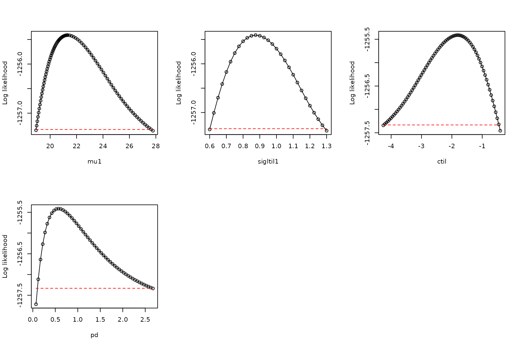

The profiles look adequate. So the model is suitable for use, unlike the previous model. The BIC and AIC for this model are valid. If the second- or third-best model is suitable in the same manner, the lowest-BIC model suitable model should tend to be preferred.

Daniel C. Reuman

Angel Luís Robles Fernández